Image Processing Algorithms Part 6: Gamma Correction

by Francis G. Loch

Gamma, represented by the Greek letter , can be described as the relationship between an input and the resulting output. For the scope of this article the input will be the RGB intensity values of an image.

The relationship is that the output is proportional to the input raised to the power of gamma. The formula for calculating the resulting output is as follows:

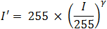
To illustrate here are a few gamma curves:

Various Gamma Curves
(click on image for full size version)

Note that with a gamma of 1 the input equals the output producing a straight line.

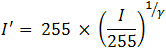
For calculating gamma correction all you need to do is raise the input value to the power of the inverse of gamma. The equation for this is as follows:

The following graph shows a comparison between the gamma curve and the gamma correction curve:

Gamma versus Gamma Correction
(click on image for full size version)

In pseudo-code performing gamma correction would go something like this:

   gammaCorrection = 1 / gamma
   colour = GetPixelColour(x, y)
   newRed = 255 * (Red(colour) / 255) ^ gammaCorrection
   newGreen = 255 * (Green(colour) / 255) ^ gammaCorrection
   newBlue = 255 * (Blue(colour) / 255) ^ gammaCorrection
   PutPixelColour(x, y) = RGB(newRed, newGreen, newBlue)

The range of values used for gamma will depend on the application, but personally I tend to use a range of 0.01 to 7.99.

Here we have the the 'Lena' and 'mandrill' images which have had the gamma corrected using a gamma of 0.25 and 2.00:

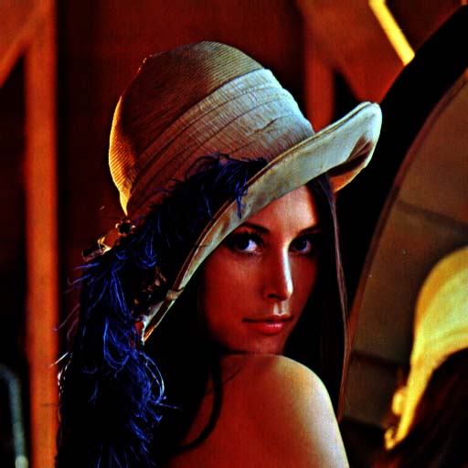
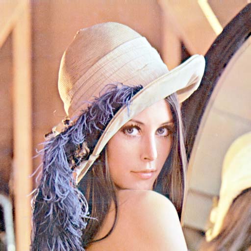
'Lena' image with gamma = 0.25	'Lena' image with gamma = 2.00

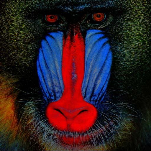
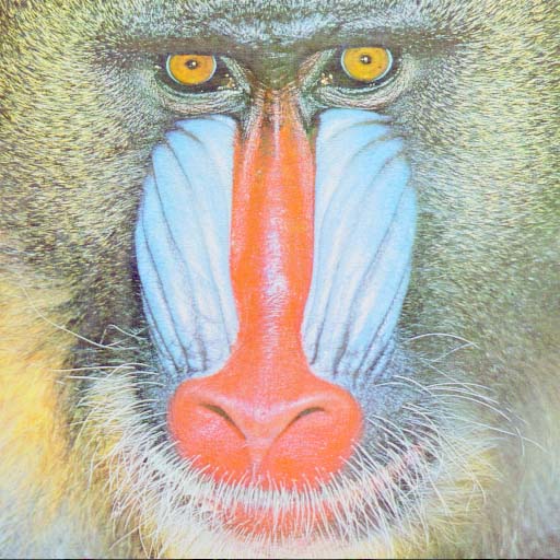
'Mandrill' image with gamma = 0.25	'Mandrill' image with gamma = 2.00